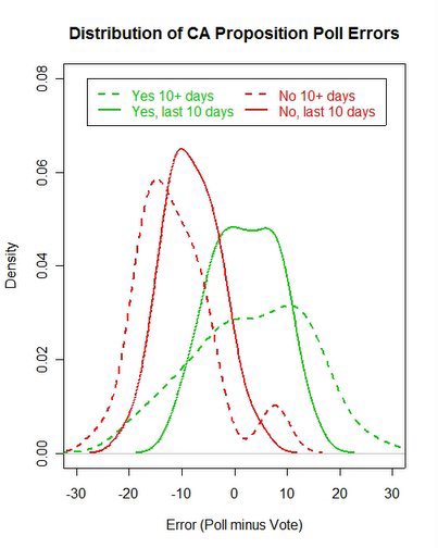
Distribution of deviations between polls and final vote on seven California referendums, November 2005.
The several California referendums this week provide a good illustration of polling variability as well as a look at the average accuracy of the polls. Earlier I illustrated the distribution of the pre-election polls here. Now that we know the results, we can compare the outcomes with the estimates from the polls.
MysteryPollster has a comparison of the polls average accuracy across the referendums here. He focuses on the mean prediction error, while I focus on the “spread” of the distribution of errors. My concern is with the uncertainty we should attach to the polls as predictions of vote. The more spread there is, the greater our uncertainty. Because the prediction error also includes all non-sampling errors, these distributions are better measures of our practical uncertainty than is the sampling error alone.
It is worth admitting up front that proposition polling is unusually difficult from a technical perspective. MysteryPollster has addressed these difficulties here (and in related posts.)
I also address the issue raised here by “sennoma” to look at the change in the error distribution between early and late polling.
The figure above shows the distribution of errors, poll minus vote percentages, pooled across all the referendums. (I omit Proposition 80 which had few polls.) The dashed lines are for polls taken more than 10 days before the vote, while the solid lines are for polls taken in the last 10 days of the campaign. The reason to pool across polls and propositions is that we have no a priori reason to assume one poll is “better” than another and no reason to assume polling is easier or harder on any given proposition. Pooling allows us to maximize cases and assess our uncertainty prior to seeing any results.
The distribution of errors tightens for polls taken in the last 10 days. For “yes” responses the middle 90% of errors from more than 10 days prior to the election range from -16.5 to +17.1. For polls taken in the last 10 days the 90% range is -8.6 to +10.6. The median error shifts from +4.1 to +1.8, showing that the middle of the distribution comes closer to the actual outcome in later polling for the “yes” vote.
For the “no” responses, the 90% range is -20.1 to +6.5 for early polling, and -16.50 to +0.55 for the last 10 days. The median error is -12.5 for early and -8.5 for late polls, showing a systematic underestimate of the “no” vote.
Put another way, the 90% confidence interval for these distributions is 19.2% for yes votes and 17.1% for no votes. That range is quite large compared to the theoretical margin of error for sample sizes typical of these surveys, which are reported to range from 3-6% for a 95% margin of error. The empirical 90% range is +/- 9.6% for yes and +/-8.55% for no votes. This inflation of theoretical margins of error by a factor of 1.5 to 2.0 or more is typical of empirical estimates of survey accuracy as predictors of election outcomes. The inflation reflects sources of error in addition to those due to sampling, such as campaign dynamics, non-response, question wording effects and other sources of error. (And since I'm comparing 95% sampling margins to 90% empirical ranges, I'm being generous to the polls here.)
These results also demonstrate the problem of bias in the survey estimates. While the percentage of “yes” votes had a median error of only +1.5, the error for no votes was a rather large -8.5% median error, a quite large error. While smaller than for early polls, the median of the “no” distribution falls rather far from the actual outcome. One might chalk this up to “undecideds” who ultimately voted no, but this is a problem of modeling from the survey data to a prediction of the outcome--- something that few pollsters actually do in public polling. (MysteryPollster calculates the errors using the “Mosteller methods” that allocate undecideds either proportionately or equally. That is standard in the polling profession, but ignores the fact that pollsters rarely adopt either of these approaches in the published results. I may post a rant against this approach some other day, but for now will only say that if pollsters won't publish these estimates, we should just stick to what they do publish-- the percentages for yes and no, without allocating undecideds.)
The bottom line of the California proposition polling is that the variability amounted to saying the polls “knew” the outcome, in a range of some +/-9.6% for “yes” and +/- 8.55% for “no”. While the former easily covers the outcome, the latter only just barely covers the no vote outcome. And it raises the question of how much is it worth to have confidence in an outcome that can range over +/- 9 to 10%? In general, I'm pretty confident elections will fall between 40% and 60%. That's only slightly larger than the empirical uncertainty in these polls. If anyone would care to pay me for that prediction, I'm pretty sure I will be as accurate as these polls. (Apologies to my pollster colleagues. But don't worry, no one will pay me for my opinion!)
The next post below (I'm posting these in reverse order) looks at polling in the New Jersey, Virgina and New York City partisan elections. These are interesting to compare to the much harder to poll proposition issues I've focused on here.
