The effects on vote of socio-economic status in the Connecticut primary are clear, though perhaps not as powerful as the chatter would suggest. (UPDATE: I've added a post using the CBS/NYT exit poll to look at individual relationships to the vote here. There is also discussion of the differences between aggregate and individual level relationships there and here.)
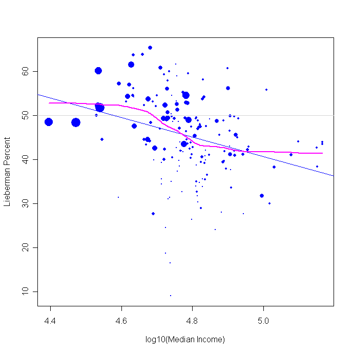
The figure above plots Lieberman vote against median household income (all data are for towns, and these are incomes from the 2000 census.) The log of income makes the relationship a little more clear than simple dollars. The relationship is a bit more linear when using log income than raw dollars. A value of 4.4 corresponds to $25,100, 4.6 to $39,800, 4.8 to $63,000 and 5.0 to $100,000.
The linear fit implies that Lamont gained about 20% more of the vote between the poorest to the richest towns, from about 45% to about 65% of the vote.
The nonlinear fit says this gain was a bit less. Below about $40,000 there was no further gain for Lieberman (or loss for Lamont). And above $63,000 there was little further Lamont gain. The action is primarily in this $40k-$63k range, in which Lieberman loses about 12%-13% to Lamont.
I think the non-linear fit is more revealing throughout these graphs, so the rest of my comments about the effects of these variables are referring to the purple local (non-linear) regression. As you can see, the effects depart quite a bit from the blue linear fits.
So the Volvo driving, latte loving Lamont voters I've been reading about is partly true. Lamont clearly does better in higher income areas. But let's not exaggerate the effect too much. Lamont got about 58% of the vote above $63k in income, which was a considerable advantage. Lieberman did just a little better than break even, winning about 52%-53% among those in towns below $40k. In between things changed rapidly with income.
Areas with increasing unemployment also helped Lieberman, but again within a narrow range.
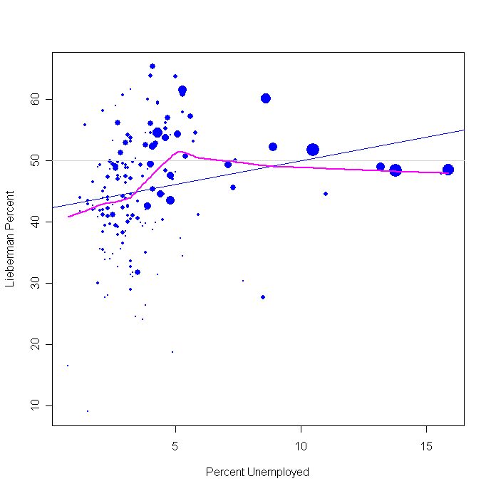
Between about 3 and 5% unemployment, Lieberman gets a fast rise in vote, but his support actually trails off as we get into the towns with the highest unemployment. The differential turnout I discussed earlier here may also account for some of this flattening. Clearly the more distressed areas were not bastions of strength for Lieberman.
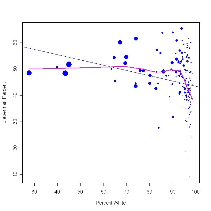
Race had a strikingly non-linear effect. The percent white has virtually no impact on Lieberman or Lamont's votes between 25% to 90% white. Throughout this range the candidates split the vote 50-50. But at white concentration above 90%, the Lieberman support takes a very sharp dive, with Lamont surging to win over 60% of the vote in the most white towns.
This race effect is largely mirrored if we look at percent black or Hispanic. The sharp non-linearity appears in both cases, though slightly shifted to the right for Hispanics compared to blacks. Once the black population reaches about 3% there are only transient gains for Lieberman.

The size of the Hispanic population shifts the Lieberman vote over a somewhat wider range, with Lieberman vote rising sharply as Hispanic population goes from 2% to 10%, but then falling back to about a 50% share of the vote for all ranges of Hispanic population above about 15%.

The bottom line is that Lamont did best in the extremely white areas and with household incomes over $63k. Lieberman managed to do relatively better (but only breaking even or a few points better than that) among the areas below $40k and with less than 90% white populations. The strong effects on vote were concentrated in towns between $40k and $63k incomes and between 90% and 100% white. Outside these ranges, there were very modest further effects of income or race.
I look at ancestry and vote in another post here.
Click here to go to Table of Contents